BigQuery Tutorial
BigQuery UI
The aim of this tutorial is to get you familiarized with BigQuery web UI to query/filter/aggregate/export data.
This tutorial is based upon one from the Google Healthcare datathon repository. It is written with the old BigQuery interface, and focuses on the MIMIC-III/eICU-CRD datasets.
Prerequisites
- You should already have had a valid Google account with access to the datasets.
- If you do not have a Google account, you can create one at http://www.gmail.com. You need to add this e-mail to your PhysioNet account.
- Access to MIMIC-III/eICU-CRD can be done via the their PhysioNet project pages.
- All users have access to the demo datasets.
PhysioNet does not cover the cost of queries against physionet-data
(though this cost is mostly trivial). In order to run queries, you will need
to configure a project for your account, which BigQuery can then use to bill
for your usage of the cloud platform. For more information on GCP projects,
see the documentation on creating and managing projects..
All PhysioNet data is hosted on the physionet-data project. You will only have
read-access privileges to these datasets. As a result, if you would like to save
the results of any queries, you will need to save them to a dataset created
on your own project.
TLDR
In this section we are going to run a query to briefly showcase BigQuery’s capability. The goal is to aggregate the mimic demo data to find out the correlation between age and the average length of stay in hours in ICU.
Run the following query from BigQuery web interface (See “Executing Queries” section above for how to access BigQuery web interface).
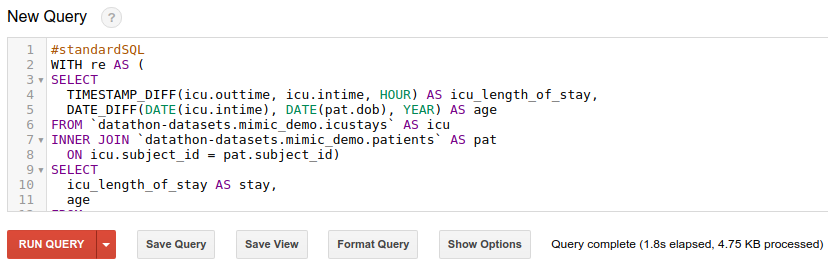
#standardSQL
WITH re AS (
SELECT
  DATETIME_DIFF(icu.outtime, icu.intime, HOUR) AS icu_length_of_stay,
  DATE_DIFF(DATE(icu.intime), DATE(pat.dob), YEAR) AS age
FROM `physionet-data.mimiciii_demo.icustays` AS icu
INNER JOIN `physionet-data.mimiciii_demo.patients` AS pat
  ON icu.subject_id = pat.subject_id)
SELECT
  age,
  AVG(icu_length_of_stay) AS stay
FROM re
WHERE age < 100
GROUP BY age
ORDER BY age
You can download the returned result as a CSV file and genereate a chart with your preferred tools.
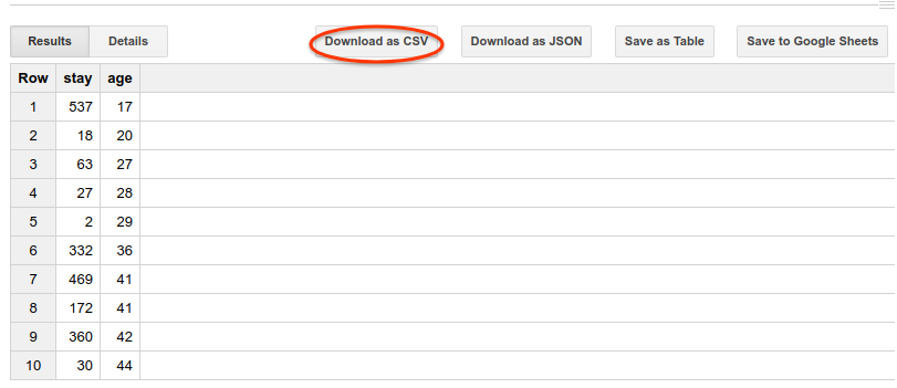
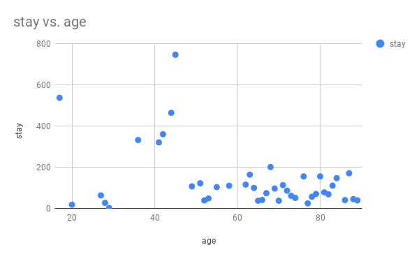
The following is a scatter chart plotted from the result with Google Sheets.
Detailed Tutorial
BigQuery Basics
Feel free to skip this section if you are already familiar with BigQuery.
BigQuery Table Name
A BigQuery table is uniquely identified by the three-layer hierarchy of project ID, dataset ID and table name. For example in the following query:
SELECT
  subject_id
FROM
  `physionet-data.mimiciii_demo.icustays`
LIMIT 10
physionet-data.mimiciii_demo.icustays specifies the table we are querying,
where physionet-data is the project that hosts the datasets, mimiciii_demo
is the name of the dataset, and icustays is the table name. Backticks (`) are
used as there is a non-standard character (-) in the project name. If the
dataset resides in the same project, you can safely omit the project name,
e.g.my-project.my_dataset.my_tablecan be written asmy_dataset.my_table
instead.
SQL Dialect
BigQuery supports 2 SQL dialects, legacy and standard. During this datathon we highly recommend using standard SQL dialect.
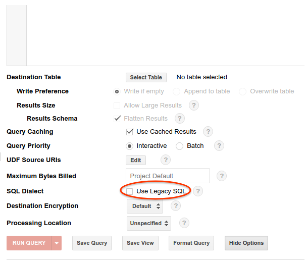
Follow the steps below to make sure the StandardSQL dialect is used:
- Click “COMPOSE QUERY” on top left corner;
- Click “Show Options” below the input area;
- Lastly, make sure “Use Legacy SQL” is NOT checked, and click “Hide Options”.
Alternatively, "#standardSQL" tag can be prepended to each query to tell BigQuery the dialect you are using, which is what we used in the TLDR section above.
MIMIC-III Basics
Dataset Exploration
As mentioned previously, the datasets are hosted in a different project, which
can be accessed
here.
On the left panel, you will see the mimiciii_demo dataset, under which you
will see the table names.
To view the details of a table, simply click on it (for example the icustays
table). Then, on the right side of the window, you will have to option to see
the schema, metadata and preview of rows tabs.
Queries
Most of the following queries are adapted from the MIMIC cohort selection tutorial.
Analysis
Let’s take a look at a few queries. To run the queries yourself, copy the SQL statement to the input area on top of the web interface and click the red “RUN QUERY” button.
SELECT
  subject_id,
  hadm_id,
  icustay_id,
  intime,
  outtime,
  DATETIME_DIFF(outtime, intime, DAY) AS icu_length_of_stay
FROM `physionet-data.mimiciii_demo.icustays`
Let’s save the result of previous query to an intermediate table for later analysis:
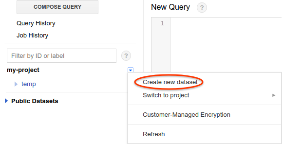
- Create a dataset by clicking the caret below the search box on the left sidebar, and choose “Create new dataset”;
- Set dataset ID to “temp” and data expiration to 2 days;
- Click “OK” to save the dataset.
- Click “Save to table” button on the right;
- Set destination dataset to “temp” and table to “icustays”, use the default value for project;
- Click “OK” to save the table, it usually takes less than a few seconds for demo tables.
Now let’s take a look at a query that requires table joining: include the patient’s age at the time of ICU admittance. This is computed by the date difference in years between the ICU intime and the patient’s date of birth. The former is available in the icustays table, and the latter resides in the dob column of the patients table.
SELECT
  icu.subject_id,
  icu.hadm_id,
  icu.icustay_id,
  pat.dob,
  icu.icu_length_of_stay,
  DATE_DIFF(DATE(icu.intime), DATE(pat.dob), YEAR) AS age
FROM `physionet-data.mimiciii_demo.patients` AS pat
INNER JOIN `temp.icustays` AS icu
  ON icu.subject_id = pat.subject_id
Again, let’s save the table as “pat_icustays” in the “temp” dataset for use later. Briefly look at the age of patients when they are admitted with the following query.
Now let’s run the following query to produce data to generate a histrogram graph to show the distribution of patient ages in ten-year buckets (i.e. [0, 10), [10, 20), …, [90, ∞).
WITH bu AS (
  SELECT
    CAST(FLOOR(age / 10) AS INT64) AS bucket
  FROM `temp.pat_icustays`)
SELECT
  IF(bucket >= 9, ">= 90", FORMAT("%d - %d", bucket * 10, (bucket + 1) * 10)) AS age,
  COUNT(bucket) AS total
FROM bu
GROUP BY bucket
ORDER BY bucket ASC
Now click “Save to Google Sheets” button and wait 1-2 seconds until a yellow notification shows up, click “Click to view” which leads you to Google Spreadsheet in a new browser window. As you can see, the data from our last query is dumped into a spreadsheet. By clicking “Insert -> Chart” from the menu bar on top, a nice histrogram graph is automatically created for us!

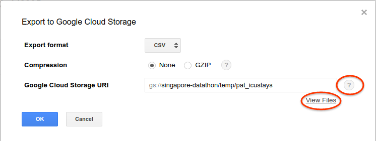
If you prefer using other tools to process the final result, a CSV file can be downloaded by clicking the “Downed as CSV” button. If downloading fails because the file is too large (we highly recommend aggregating the data to a small enough result before downloading though), you can save it to a temporary table, click the caret then “Export table” button from the dropdown menu and save it to Google Cloud Storage, then you can download the file from GCS.
Now let’s see if there is correlation between age and average length of stay in hours. Since we are using the age of patients when they get admitted, so we don’t need to worry about multiple admissions of patients. Note that we treat the redacted ages (> 90) as noises and filter them out.
WITH re AS (
SELECT
  DATETIME_DIFF(icu.outtime, icu.intime, HOUR) AS icu_length_of_stay,
  DATE_DIFF(DATE(icu.intime), DATE(pat.dob), YEAR) AS age
FROM `physionet-data.mimiciii_demo.icustays` AS icu
INNER JOIN `physionet-data.mimiciii_demo.patients` AS pat
  ON icu.subject_id = pat.subject_id)
SELECT
  icu_length_of_stay AS stay,
  age
FROM re
WHERE age < 100
Follow the same steps to save the result to Google Spreadsheet, by default a linear chart is generate. We will need to change the chart type to scatter chart through the chart editor on the right.
Useful Tips
Saving View
Datathon organizers might not allow you to create new tables. However, you can save a view of a query’s output to then use in later queries.
-
Create a temporary dataset in the datathon project. Next to the datathon project in the left side of the BigQuery UI, click the arrow and then
Create new dataset. Give the dataset a temporary name that can be identified to your team (like ‘team6temp’). -
Save the view. After running your query, click the button next to
Run Querythat saysSave view. Select the temporary dataset you created and then give the view a name. -
Query your view. Now you can perform a query using the syntax
project.dataset.viewlike the following:SELECT * FROM `datathon_project.team6temp.our_custom_view`;
Working with DATETIME
The times in the tables are stored as DATETIME objects. This means you cannot use operators like <, =, or > for comparing them.
-
Use the DATETIME functionsin BigQuery. An example would be if you were trying to find things within 1 hour of another event. In that case, you could use the native DATETIME_SUB() function. In the example below, we are looking for stays of less than 1 hour (where the admit time is less than 1 hour away from the discharge time).
[...] WHERE ADMITTIME BETWEEN DATETIME_SUB(DISCHTIME, INTERVAL 1 HOUR) AND DISCHTIME -
If you are more comfortable working with timestamps, you can cast the DATETIME object to a TIMESTAMP object and then use the TIMESTAMP functions.
Input / Output Options
There are a few cases where you may want to work with files outside of BigQuery. Examples include importing your own custom Python library or saving a dataframe. This tutorial covers importing and exporting from local filesystem, Google Drive, Google Sheets, and Google Cloud Storage.
Closing
Congratulations! You’ve finished the BigQuery web UI tutorial. In this tutorial
we demonstrated how to query, filter, aggregate data, and how to export the
result to different locations through BigQuery web UI. If you would like to
explore the real data, please use mimiciii_clinical as the dataset name. For
example, the table mimiciii_demo.icustays becomes mimiciii_clinical.icustays
when you need the actual MIMIC data. Please take a look at more comprehensive
examples here such as creating charts and training
machine learning models in an interactive way (or copy the queries over to web
UI to execute if you prefer) if you are interested.
Feedback
Was this page helpful?
Glad to hear it! Please raise an issue here to tell us how we can improve.
Sorry to hear that. Please raise an issue here to tell us how we can improve.